Weak lensing mapping

Science with weak lensing mappings
Survey goals with cosmic variance estimates
Interactive choice of configuration
Dependence with the cosmological parameters
_
Science with weak lensing mappings (back to top)
(see a detailed presentation of these calculations in the paper "Weak Lensing Statistics as a Probe of Omega and Power Spectrum" by Bernardeau et al. 1997)


Distortion maps provide maps of projected mass: the local convergence field is proportional to the integrated density along the line-of-sight, from the observer to the source plane with an efficiency that depends on geometrical factors. More precisely we have,

that relates in a given direction to the overdensity. This relation makes intervene the integral along the radial distance and depends on the cosmological parameters through the angular distances and mainly through the overall factor . This factor betrays the fact that fundamentally the local convergence is a measure of the total density and not of the overdensity. The above relationship is dimensionless when the angular distances are expressed in units of . 
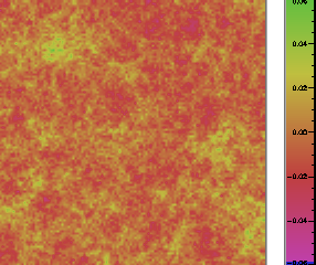
The elaboration of a distortion map would permit the determination of statistical quantities related to the cosmic density field. The easiest quantity to get is the rms convergence. It is directly proportional to the spectrum normalisation, , and, at the degree scale, it reaches values of the order 1%,
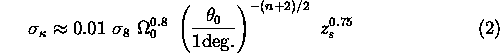
.

Obviously then amplitude depends on the mean redshift of the sources (the further the sources are, the larger the effects are) and on the the value of (however the result is not directly proportional to because of the growing rate of the fluctuations). 
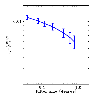
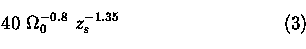
These maps would allow also to estimate the degree of non-linearities that have been reached by the dynamics. This is a means to separate the determinations of and of . Indeed for a given amplitude of the convergence fluctuations, the smaller is, the larger should be. 
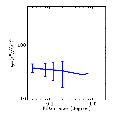
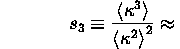
As a result, the convergence field is expected to exhibit non-Gaussian features (assuming that the initial conditions were Gaussian) that are all the more important that is small. A classic way of quantifying those effects is to consider the skewness, third moment of the probability distribution function of the local convergence expressed in units of the square of the second moment. One expects this quantity to be finite. The perturbation theory applied to the growth of structures predicts

The skewness appears to be way of measuring independently of the amplitude of the fluctuations.
_

Survey goals with cosmic variance estimates (back to top)
(see a detailed presentation of these results in the paper "Efficiency of weak lensing surveys to probe cosmological models" by van Waerbeke et al. 1999 and a recent extension of these results to the nonlinear regime in "Weak Lensing Predictions at Intermediate Scales" by L. Van Waerbeke (CITA, IAP), T. Hamana (IAP), R. Scoccimarro (IAS), S. Colombi (IAP, NIC), F. Bernardeau (SPhT, Saclay). )


We have built synthetic maps that reproduce the level of signal and of noise that is expected in realistic cosmological models.

We present here an example of such a synthetic random map: for each selected configuration (see next paragraph), the presented map corresponds to the same set of random numbers. They are all 5x5 square degree large. The pixel size is 2.5 arcmin^2.

A realistic level of non-linear couplings is introduced with a second order Lagrangian approximation. The latter is directly applied to the projected mass map. The corresponding shear maps are then calculated after the the projected gravitational potential has been built. A realistic noise due to the intrinsic ellipticities is added at this stage. It corresponds to the source number density of either 30 or 50 gal/arcmin^2.

We then have at our disposal a set of maps that reproduces as reliably as possible what a realistic survey would be. Eventually the mass map is built with a maximum likelihood method (applied once again to the gravitational potential). One recovers almost all the structures that were present. The noise is predominant at the pixel scale only.


For each of these maps we have computed the moments of the one-point PDF. Two quantities have been examined: the variance (first panel) and the skewness (second panel). The error-bars representing the cosmic variance have been obtained with 60 realizations of each model.

_

Interactive choice of configuration (back to top)


The results that are presented here are for a somehow standard configuration. The default set of parameters can be changed to appreciate how it is affected by the cosmological parameters.
for the choice of Cosmology
The possibilities that are available correspond to either a power spectrum found to fit the APM angular survey (Baugh and Gaztanaga, henceforth "BG" spectrum) for either an Einstein-de Sitter Universe or Omega=0.3, Lambda=0 Universe or a standard CDM model. In some cases several values of sigma_8 are proposed.

for the redshift of the sources

In our calculations the sources are assumed to be all at the same redshift. This is a valid approximation as long as the redshift distribution is sufficiently narrow. The mean redshift of the sources that have been considered are either 1 or 1.5.

for the mean number density of sources

The precision of the measurements at small scales depends on the mean number density of galaxies for which a reliable estimation of the ellipticities can be done. This number density depend on both the depth of the survey and on the instrumental precision.
In the paper van Waerbeke et al. (1998), we have shown that the noise due to the intrinsic ellipticities was equivalent to a shot noise. We propose in the options to consider either the case of the continuous limit, the case of either 30 or 50 galaxies/arcmin^2
for the size of the survey.
The cosmic variance of the results depends on the area and geometry of the survey. So far we have results available for a compact square survey only. The sizes ranges from 2x2 degree^2 to 10x10.


for the choice of filter.
_

Dependence with the cosmological parameters (back to top)


The following table gives an idea of the expected constraints for a realistic cosmologial scenario. One can see that for a 10x10 square degree survey, a very interesting precision can be reached for the skewness and therefore for .


models = 1 = 0.3
5x5 deg, zs=1 50 gal/arcmin^2 0.051 0.190 0.047 0.118
30 gal/arcmin^2 0.050 0.186 0.047 0.105
5x5 deg, zs=1.5 50 gal/arcmin^2 0.0430.2460.0380.127
30 gal/arcmin^2 0.0430.2230.0380.123
10x10 deg, zs=1 50 gal/arcmin^2 0.0290.1160.0240.050
30 gal/arcmin^2 0.0290.1100.0230.054

The constraints on the skewness significantly depend on the cosmological constant. When this is taken into account the following constraints are obtained: in red corresponds a large value for the skewness, in blue a low value (1 or 2 sigma constraints for each case). The left panel is for a 5x5 square degree survey, the right panel for a 10x10 survey.