4.4 Photometric accuracy

In this Section we attempt to make a robust estimate of the internal photometric errors of the CFHTLS using a variety of methods. Although Scamp provides an estimate of the internal photometric error (between individual MegaCam images), we instead focus on the photometric errors in the final tiles. This way, initial calibration errors and any other subsequent source of errors, inside each stack and field-to-field are better taken into account, leading to a more realistic estimation of the errors.

4.4.1 Internal photometric errors of Wide stacks from simulations

The internal photometric errors are derived using the same simulations used in the completeness analysis described in Section 4.3. The use of simulations enables a better control of the input and output sources and ensures that all Wide stacks are evaluated consistently. As before, simulated sources are added to the real T0007 Wide stacks and processed the same way as real sources. Their photometry is then compared to the input simulated values. The simulated sources are added within the central 10000×10000 pixel and consequently are expected to be free from edge effects.

This procedure has been applied to the 855 Wide stacks, using simulated stars generated on a grid of FWHM in steps of 0.05′′ using the Skymaker software (?). In each case, stars with a FWHM closest to the stack in question are selected. For each sample, the magnitude difference between the input and the output simulated sources as a function of magnitude is computed and the FWHM of the magnitude distribution is derived after 3-σ clipping. The internal error is then given by σ_mag =FWHM/2.35 .

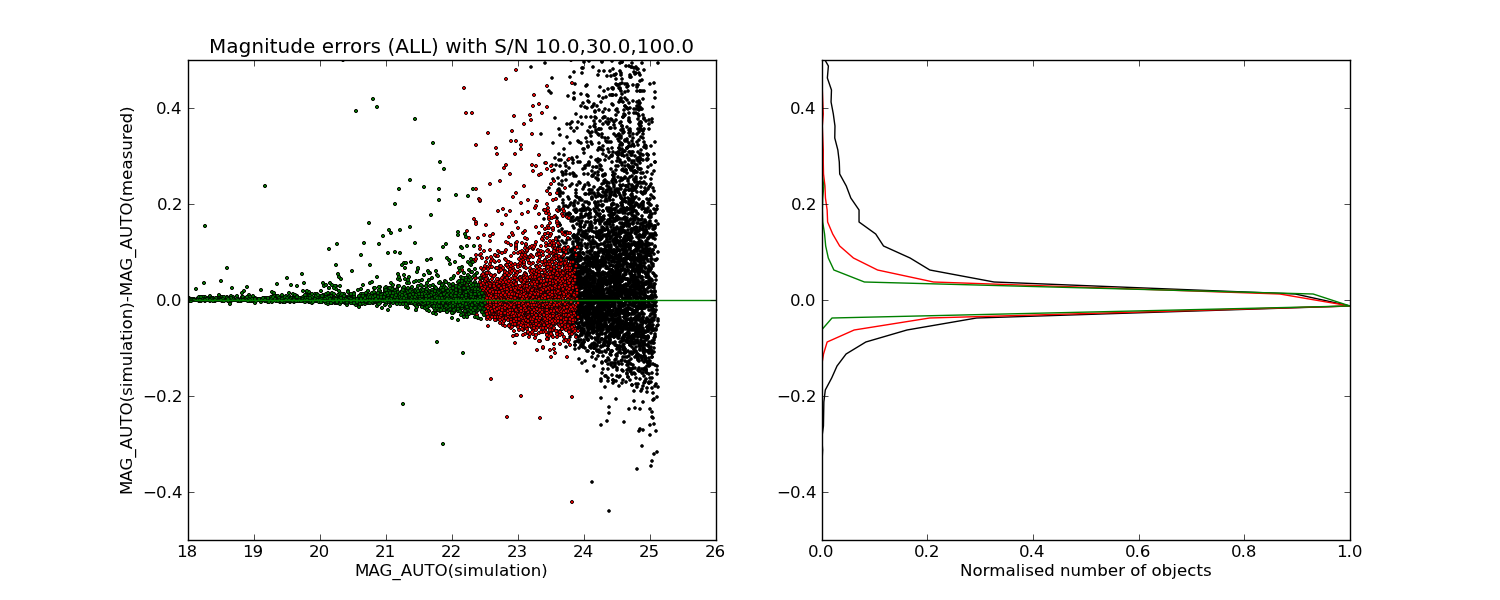
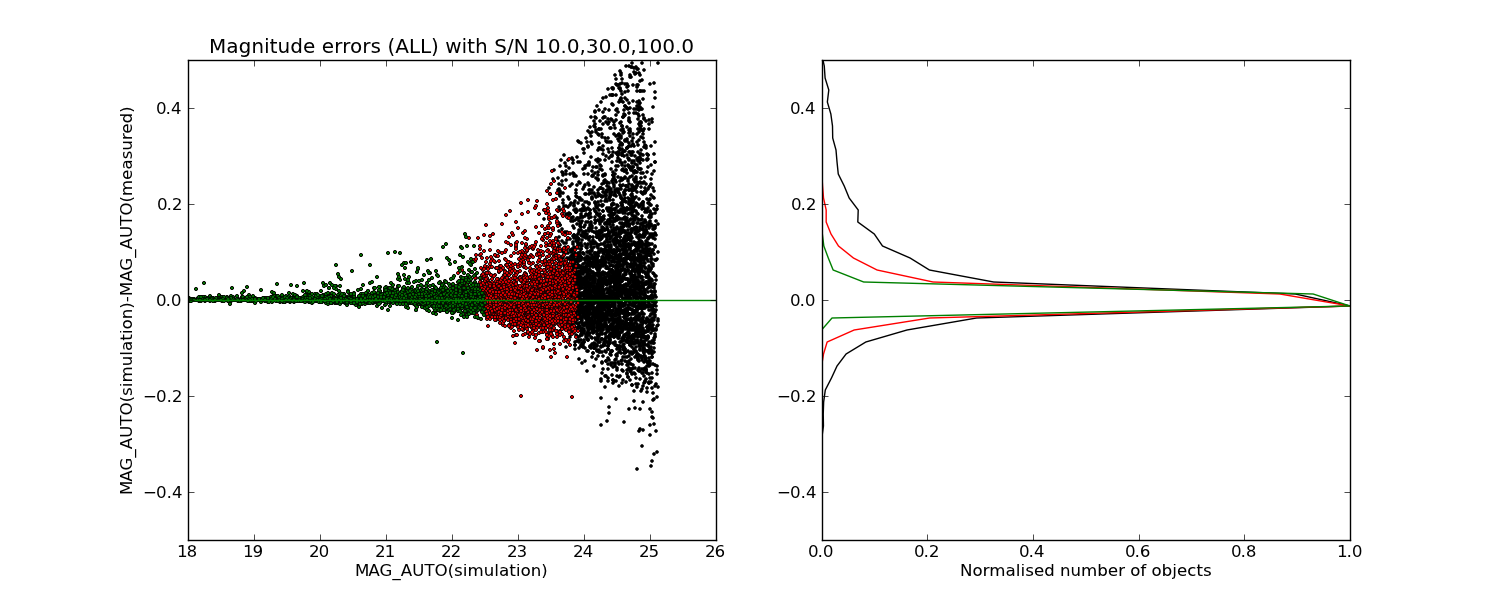
Error estimates are computed for sources selected with signal-to-noise ratios of 10, 30 and 100, respectively, or as a function of magnitude Fig. 34 shows an example result for internal photometric analysis of the CFHTLS T0007 Wide stack CFHTLS_W_g_020241-041200_T0007. The statistics compare the MAG_AUTO magnitude calculated by SExtractor for several thousands of stellar sources. It is interesting to note that the results are very stable down to signal-to-noise values of 10. Note that the difference between the input and output magnitudes as function of magnitude is not flat, but tilted. The tilt may artificially increase the dispersion inside a magnitude bin and may contaminate the internal error estimates, if the bin is large. The mean inside a bin is then corrected from the tilt prior to deriving an errors or FWHM.

The internal errors per magnitude bin are listed in Table 7.

Wide Field Magnitude range u* g r i y z [MegaCam AB] [mag.] [mag.] [mag.] [mag.] [mag.] [mag.] W1 0.002 0.002 0.003 0.006 0.003 0.008 0.005 0.003 0.010 0.007 0.007 0.017 0.008 0.009 0.011 0.016 0.014 0.043 0.020 0.015 0.025 0.037 0.035 0.098 0.046 0.035 0.061 0.089 0.083 0.159 W2 0.002 0.002 0.003 0.003 - 0.009 0.004 0.004 0.005 0.007 - 0.018 0.009 0.009 0.012 0.016 - 0.041 0.020 0.016 0.027 0.038 - 0.097 0.050 0.038 0.067 0.087 - 0.161 W3 0.002 0.001 0.002 0.003 0.002 0.008 0.004 0.003 0.005 0.007 0.007 0.018 0.008 0.007 0.011 0.017 0.015 0.040 0.020 0.015 0.025 0.039 0.034 0.095 0.049 0.035 0.060 0.094 0.084 0.140 W4 0.002 0.001 0.002 0.003 0.003 0.009 0.004 0.003 0.005 0.007 0.007 0.019 0.008 0.007 0.013 0.017 0.015 0.044 0.020 0.015 0.028 0.041 0.035 0.098 0.049 0.035 0.057 0.094 0.088 0.142 Table 7: Internal photometric errors per magnitude bins derived for each CFHTLS Wide field. The simulated sources include only stars and are detected and analyzed in the same was as real sources. The errors are the fwhm/2.35, as shown in Fig. 34. They are corrected from the amplitude of the tilt from horizontal of the difference between of the input and output magnitudes as function of magnitude inside the bin. The magnitude ranges quoted in the table only comprise bins with all sources below the completeness limits and with all sources having a signal-to-noise ratio larger than 10. The W2 y-band is not quoted because it only concerns two stacks and the statistics are meaningless for these fields.

Figure 34: Analysis of the internal photometric errors in CFHTLS_W_g_020241-041200_T0007 using simulations of stars. The top panels are analyzed without clipping and the bottom panels after a 3-σ clipping. The figures show the results for three sub-samples selected from signal-to-noise ratio (not magnitudes): S/N=10 (black), 30 (red) and 100 (green). Each panel is split into two plots. On the left the magnitude differences between the true input and the measured output magnitudes of simulated sources are drawn as a function of magnitude. The sub-samples are shown in green, red and black colors. On the right, the normalized distributions for the three sub-samples are shown. The FWHM, errors, σ=fwhm/2.35, in table 7 are derived from the histograms. Note that a magnitude dependant offset has been corrected prior to computing the FWHM and the errors inside a magnitude bin quoted in Table 7.

4.4.2 Error estimation from overlapping Wide tiles

An estimation of the internal photometric errors of the Wide survey can also be made using common sources in overlapping tiles. Since each tile is shifted by 56′in RA and 57′in DEC with respect to its nearest tiles overlap regions are stripes of 4′ × 60′ or 3′ × 60′ (see Fig. 21). We use the u^*, g, r, i and z-band MAG_IQ20 stars located in these regions to compare the photometry of sources detected in two adjacent stacks. The analysis is restricted to stars to avoid the specific issues involved in the use of MAG_AUTO for galaxies. Furthermore, it can only be applied on thin strips located at the edges of images where sources have lower signal-to-noise due to the adopted dithering strategy; therefore, this analysis should be regarded as secondary to our previous simulation-based estimations.

The first estimate of internal errors is derived by calculating for each pair of overlapping tiles the median of the magnitude differences of all source pairs in the overlapping regions. This value is the field to field photometric offset between the two contiguous tiles. For a complete Wide patch, the standard deviation of these field to field offsets is a estimator of the field to field scatter. The values for each field and filter are listed in Table 8. To compare these errors with estimators calculated from a comparison to a reference catalogue used in Section 4.4.3, a hypothesis has to be made on the distribution of this random variable. If we assume that photometric measurement are Gaussian-distributed around the “true” photometry with a dispersion of σ, then the dispersion of the field to field offsets is a Gaussian with a dispersion σ. The values of Table 8 must be divided by to be compared with the field to field estimations of Table 11. The errors are larger in u^* and z bands for several reasons: the residuals from fringe subtractions in z, the poorer image quality in u^*, especially at the edges of the stacks, and the residuals from the internal calibration errors. Considering the factor of , these errors are completely consistent with an overall photometric field to field scatter of 1% in g,r and i and 1.5% in u^* and z.

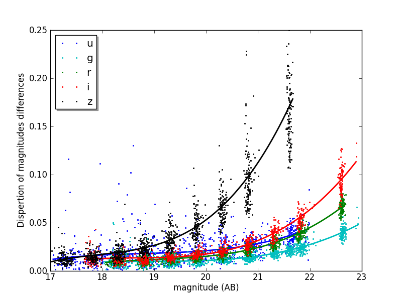
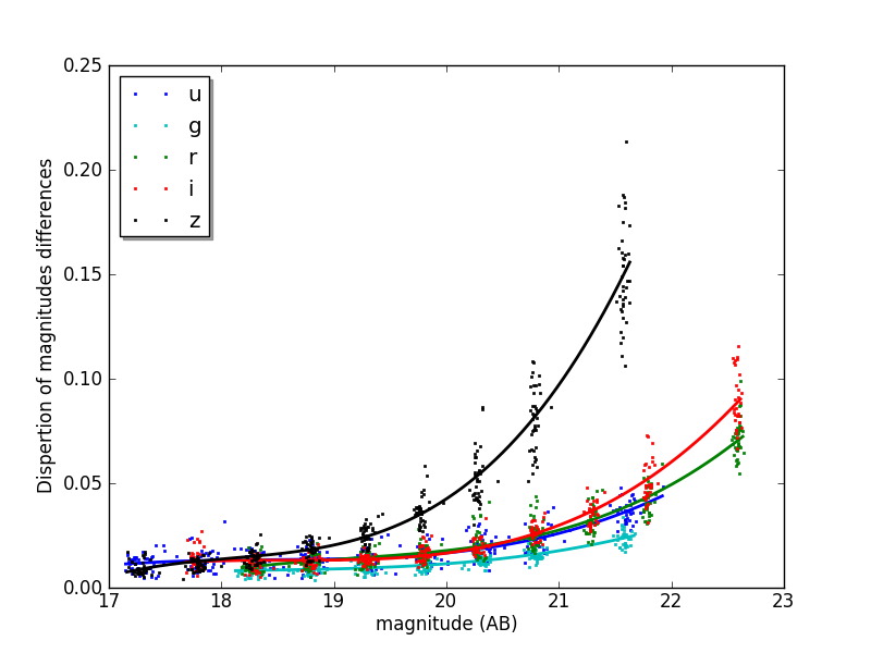
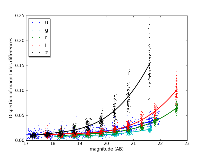
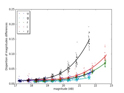
The second estimate of internal photometric errors which can be determined from the analysis of objects observed in multiple tiles is the measurement error. Since the images are photometrically flat, the dispersion of the magnitude offsets around the mean field-to-field shift of objects detected in multiple tiles is dominated by statistical measurements errors. This dispersion as a function of magnitude is plotted as the vertical error bars in Figure 35 for each of the four Wide patches and is listed in Table 9. In this analysis, both stars and galaxies are included; magnitudes are estimated using MAG_AUTO to yield a realistic estimate of measurement errors for both stars and galaxies. We also note the plots are broadly similar for each of the four patches, confirming the homogeneous nature of the Wide survey. The z-band errors are several times higher that other bands; for these longer wavelengths fringing residuals become an true issue.

The dispersion distributions are fitted with third order polynomials. To compare these values to the direct estimation of measurement errors in the simulations, one has to assume a gaussian distribution (dispersion σ_M) of the measured magnitude around the true magnitude. The distribution of the magnitude differences is then a Gaussian distribution with a dispersion equal to :

(13)

These errors are listed in Table 9.

Wide Field Magnitude range u* g r i z [MegaCam AB] [mag.] [mag.] [mag.] [mag.] [mag.] W1 0.013 0.007 0.009 0.010 0.025 0.016 0.008 0.013 0.016 0.054 0.024 0.014 0.023 0.031 0.112 0.039 0.026 0.043 0.062 0.210 0.065 0.046 0.078 0.114 0.359 W2 0.010 0.006 0.010 0.009 0.020 0.014 0.009 0.015 0.015 0.045 0.024 0.016 0.025 0.030 0.100 0.043 0.027 0.047 0.059 0.195 0.074 0.044 0.083 0.108 0.344 W3 0.011 0.007 0.009 0.010 0.023 0.016 0.009 0.013 0.016 0.049 0.025 0.014 0.022 0.033 0.101 0.040 0.023 0.043 0.066 0.189 0.062 0.036 0.079 0.123 0.324 W4 0.008 0.006 0.008 0.010 0.019 0.012 0.008 0.013 0.016 0.044 0.023 0.013 0.024 0.031 0.097 0.044 0.022 0.046 0.061 0.189 0.079 0.036 0.083 0.111 0.332 Table 9: Internal photometric errors per magnitude bins derived for each cfhtls Wide field. The magnitudes of the objects detected in two stacks are compared. For each pair of stacks, a mean offset and dispersion is calculated from the magnitude differences of each pair of objects. Assuming a gaussian distribution of errors, the listed values are estimated as the dispersion divided by .

Comparing these errors with those derived from the simulations shows that the errors from the overlaps are larger. This is to be expected and can be explained by several reasons: the statistics on the objects in the overlaps rely on sources detected at field edges where image quality and signal-to-noise is lowest due to dithering and PSF degradation at the edge of the field. Furthermore, the flatness of the photometry across the field of view show a departure from the reference central photometry on the very edges. This effect is slightly non-symmetric and affects the reliability of the magnitude measurements at the field edges. Therefore these error estimates should be considered as upper limits and contain residual systematic effects which add to the pure statistical flux measurement errors.

a href="figs/W4_dispmag.png"> Figure 35: Magnitude errors as a function of magnitude derived from sources from overlapping regions for W1, W2, W3 and W4 (top left and top right and bottom left and bottom right fields respectively).

4.4.3 Comparing CFHTLS-T0007 with SDSS-DR8

As a further check of our reduction and calibration procedures we wish to compare photometric measurements on the CFHTLS Wide with an external and well-characterized survey. Our aim is to check both the relative tile-to-tile calibration and the absolute photometric calibration. At the present time, the best candidates are the surveys conducted using the Sloan telescope at Apache Point Observatory. The latest release of the main Sloan survey, SDSS-DR8, overlaps at least partially with all four Wide patches of the CFHTLS.

As thoroughly documented in Betoule et al. (submitted), the final release of the SNLS (SNLS5) compares in absolute to the SDSS Supernova Survey on Stripe 82 at better than 1% in the griz bands, and 2% for the u^* band. The MegaCam to SDSS transformation provided below for all MegaCam filters is based on that specific effort. The MegaCam T0007 photometry is exclusively in the AB system (?). The following offsets used to convert the SDSS AB magnitude to the MegaCam AB magnitude are based on values presented in Table 1 from ?, derived from observed and synthetic measurements of Solar analogs for the SDSS Supernova Survey. They have been produced in narrow color ranges.

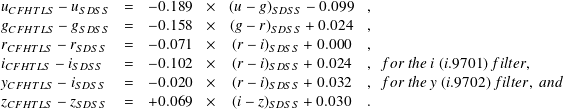(14)

It is important to realize the SDSS Supernova Survey on the SDSS Southern equatorial stripe 82 (SS82) is the result of a different effort from the general SDSS survey, the SDDS-DR8 catalogue as of 2012, to which the T0007 is being compared to in this section. The two SDSS surveys follow different calibration paths. From the joint effort between the SNLS and the SDSS Supernova Survey, that survey is known for being precisely anchored in a true AB system. This is however not the case for the general SDSS survey which is known to suffer from systematic offsets to a true AB system²³ , while the internal relative photometry of the SDSS-DR8 across the sky is about 1% in gri and about 2% in u and z, the systematic offsets in respect to the true AB system are known to be larger:

In consequence, one should expect systematic residuals when comparing T0007 to SDSS-DR8 using the present transformation equations established on the the true SDSS AB system. To assess this fundamental differences between SDDS SS82 (to which the SNLS compares at better than the percent) and SDSS-DR8, we compared the offsets between the magnitude of the SNLS tertiary standards located on two Deep fields which overlap with SDSS-DR8 (D2 and D3 CFHTLS fields). We found the following offsets for the difference between the true MegaCam-AB magnitude of the SNLS tertiary standards (including their conversion from their published Vega magnitude to AB) and the SDSS-DR8 magnitudes of the SNLS tertiary standards converted to the MegaCam-AB system using Equation 14:

• -0.033 to -0.055 offset in u^*
• less than 1% offset in g,r,i
• +0.000 to +0.011 offset in z

Based on the photometric consistency of the CFHTLS Wide with the Deep/SNLS, such systematic offsets should in consequence be found between the Wide and SDSS-DR8. A generous 115 amongst the 171 Wide fields have sources in common with SDSS on all four Wide patches. As in previous releases, the photometric calibration has been verified by comparing the CFHTLS and SDSS bright sources in regions where the SDSS-DR8 overlaps with the Wide fields.

The CFHTLS and SDSS-DR8 sources have been cross-identified using the public SDSS catalogue (Data Release 8; http://www.sdss.org) and the mag_auto magnitudes of the CFHTLS merged source catalogue. The CFHTLS and SDSS photometry data have been compared using a well-defined common sample bright stars in unmasked regions of CFHTLS stacks. For W1, W2 and W3, only unsaturated stellar objects with 17 < i < 21 (i.e the limiting magnitude for a clear star/galaxy separation) located inside a cross-identification radius of 2′′ have been used. For W4, which is more contaminated by very bright stars, we only used stellar sources with 17 < i < 20.

Figure 36: Distributions of photometric offsets, δm=u*,g,r,i∕y,z, between CFHTLS Wide and SDSS-DR8 for W1, W2, W3 and W4.

The mean offset for the m-band inside a MegaCam field, δ_m, is calculated using a weighted mean :

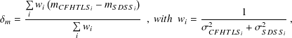(15)

where i is the index for each common star, m_i denote the magnitudes, and σ_i the magnitude errors as listed in the CFHTLS and the SDSS catalogues. Note that the offsets calculated here are averaged over a full MegaCam field.

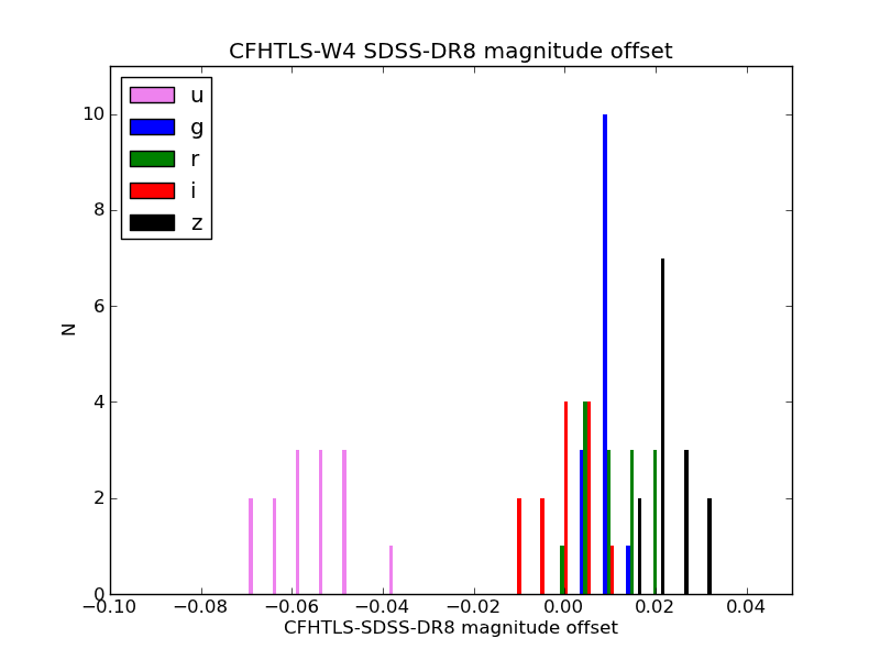
From this star sample, we define two different mean magnitude offset values, depending on the angular scale over which the offset is averaged:

• the 115 mean offsets, δ_{m=u^*,g,r,i∕y,z}, averaged over a MegaCam field. They are computed for all stacks with common stars between T0007 and SDSS-DR8. The offset values are listed in the appendix as well as in the synoptic table.
• the W1, W2, W3 and W4 offsets, averaged over each Wide field, ⟨δ_{m=u^*,g,r,i∕y,z}⟩. They are summarized in Table ?? and in the histograms of Figure 36;

The external photometric errors are then derived by applying the 115 mean offset values for each tile and by computing the rms of the distribution. The results are presented in the next section following the discussion of magnitude offsets.

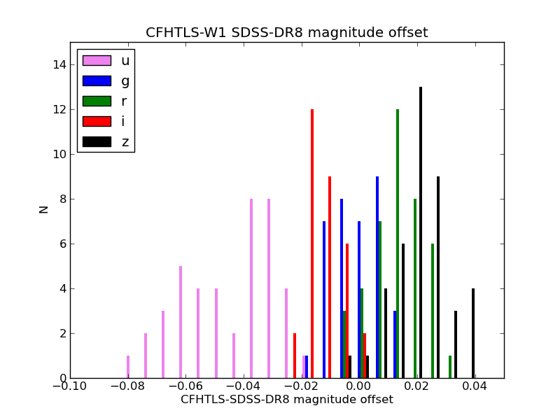
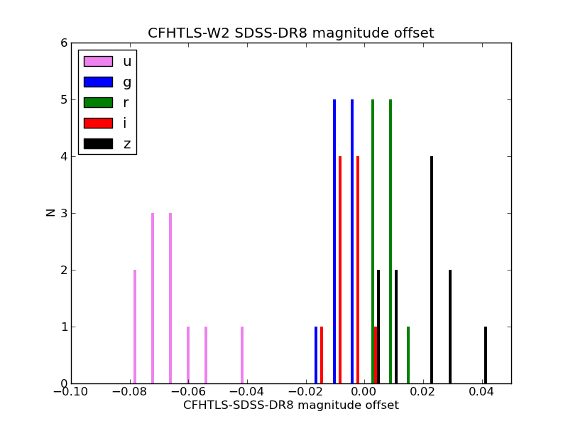
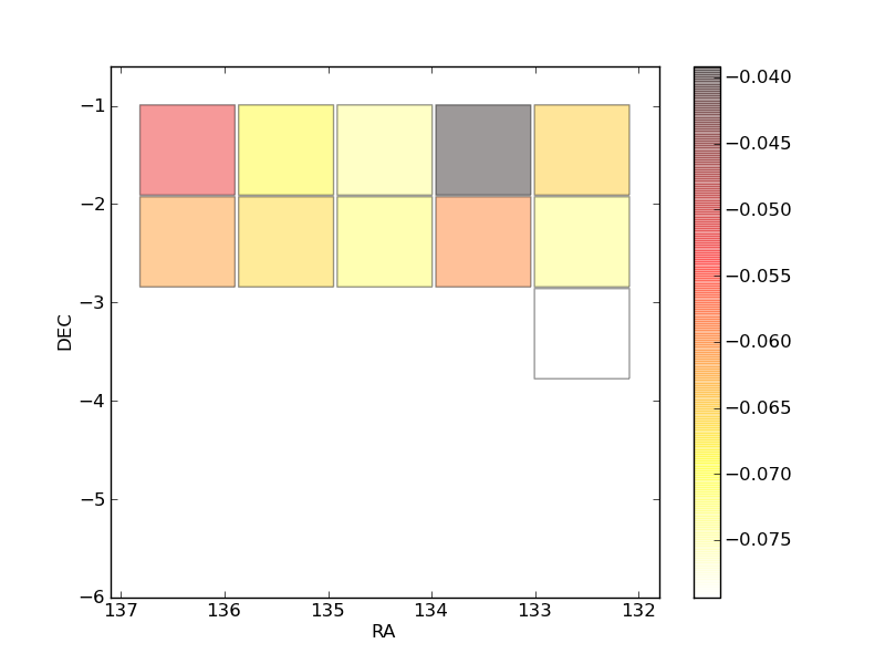
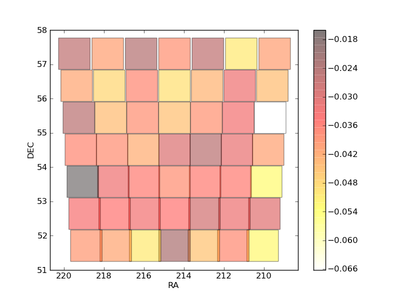
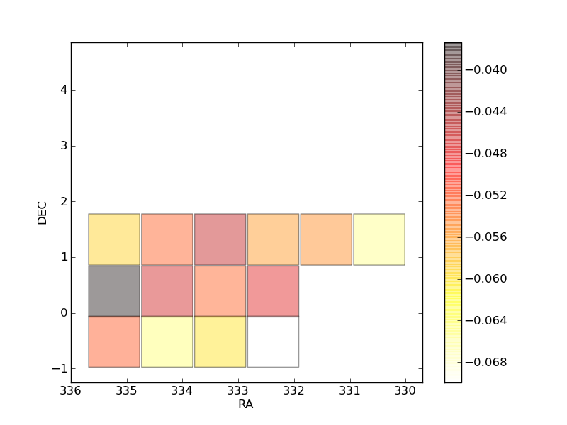
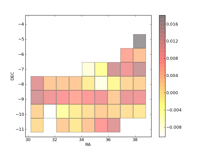
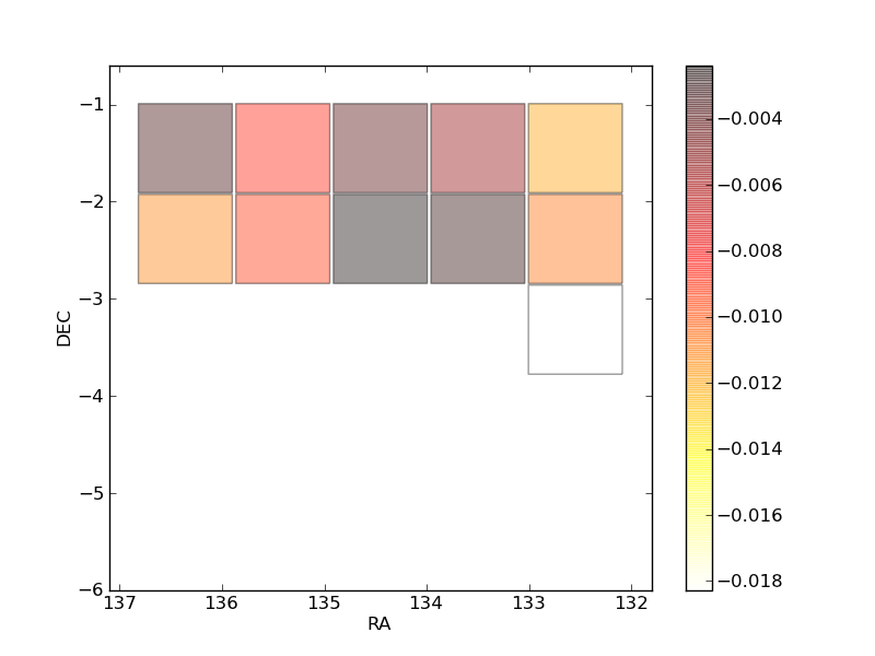
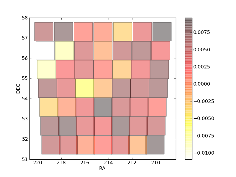
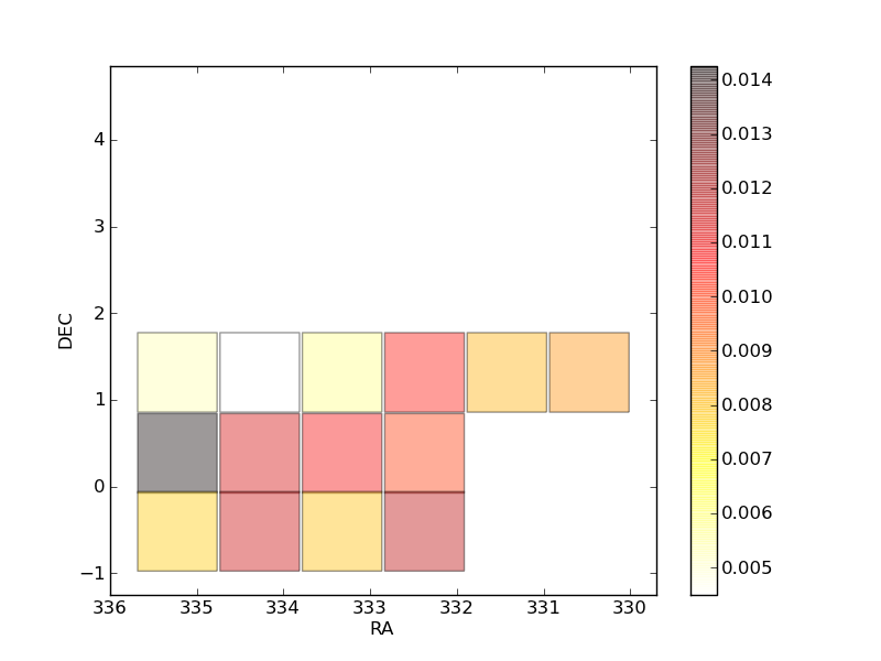
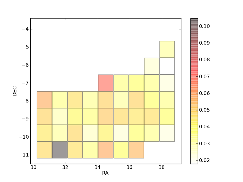
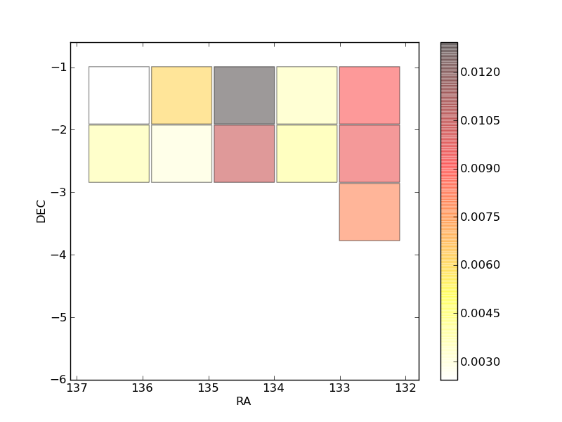
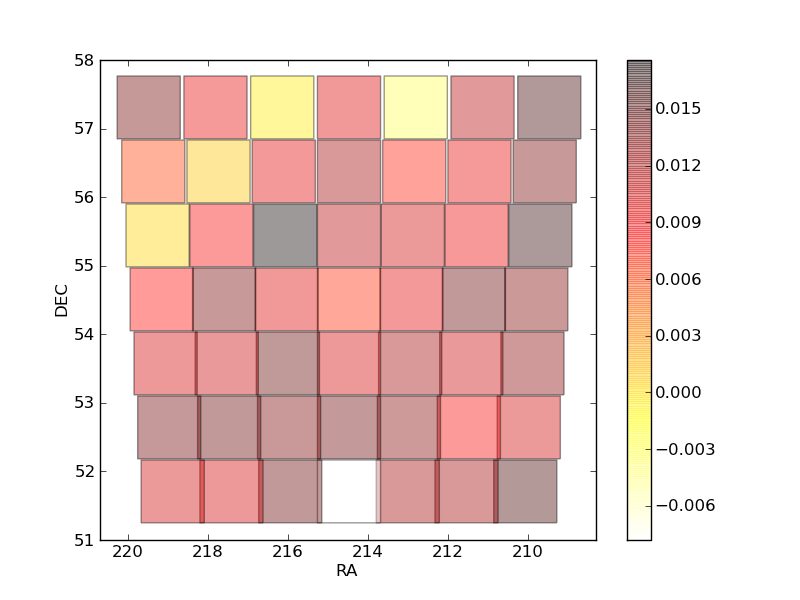
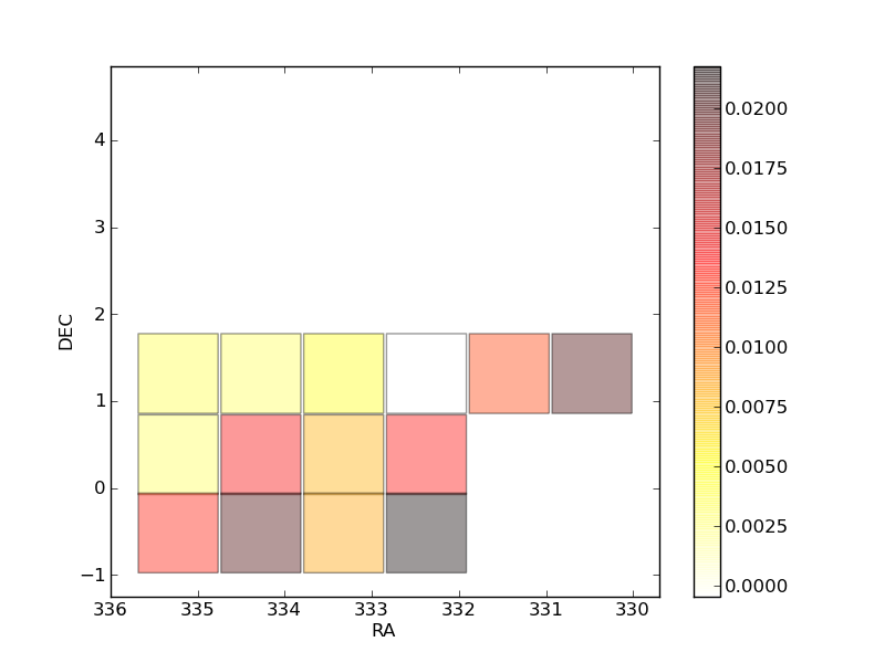
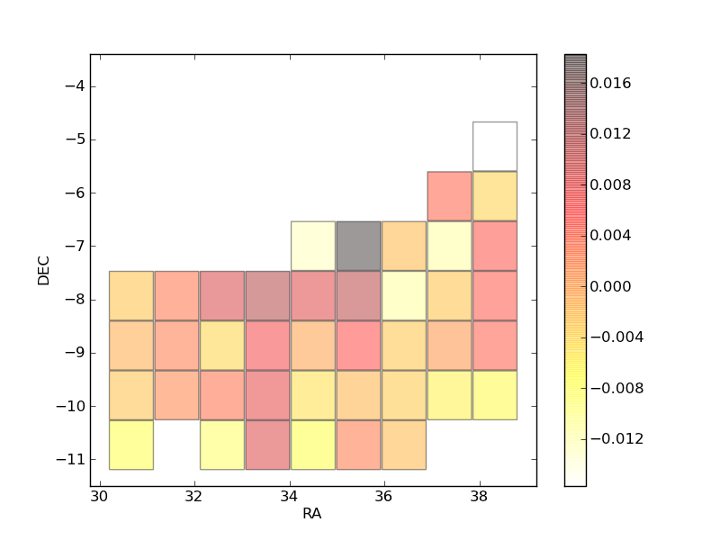
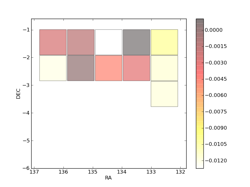
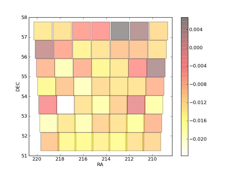
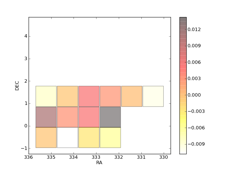
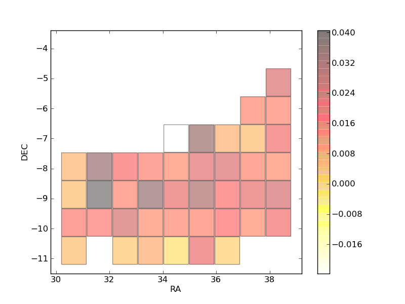
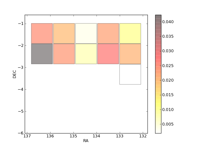
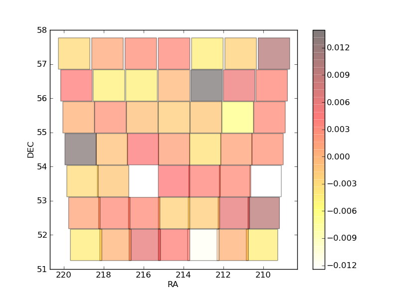
Fig. 36 separates W1, W2, W3 and W4. There is no significant difference between the four fields: the histograms show that the mean and rms offset values are consistent from field to field in all bands. The u^* and z bands exhibit however a stronger dispersion than the g, r, i bands. Table 10 presents this histogram data averaged per Wide patch: the expected offset between T0007 and SDSS-DR8 is found in the u^* band (-0.05 mag on average) and the z band (+0.02 mag) while the g,r,i bands exhibit an offset lower than 1%. Identifying these systematic offsets between SDSS-DR8 and the MegaCam AB system confirms the proper photometric bootstrapping of the Wide patches.

The higher offset found in the u^* and z bands (resp. 5% and 2% compared to less then 1% for g,r,i) is also in line with the uncertainty estimates of the SNLS tertiary standards calibration. The respective contributions to these discrepancies from the SNLS and the SDSS is still unclear. We remind that the anchoring of the DR8 to AB is thought to be off by about 0.04mag. The precision of the z band calibration precision is limited by the precision of the color transformation of BD+17.4708 at the 2% level. The larger offset seen in the u^* band stems from the fairly significant difference between the filters used in those two cameras, coupled to the large spectral range of stars used as calibrators.

Figure 37: Maps of photometric offsets between CFHTLS Wide and SDSS-DR8, based on stars common to both surveys (115 Wide stacks). Each square represents a 1o ×1o tile (or a stack) of the CFHTLS Wide. The top panels show, from left to right, the u*, g, r, i∕y and z magnitude offsets for W1. The middle panels are the same for W2 and W3, and the bottom for W4.

4.4.4 External photometric errors

The external photometric errors are derived from the rms of the mean cfhtls-sdss magnitude offset values, δ_{m=u^*,g,r,i∕y,z}, in each Wide field separately. They are measured by adding the 115 offsets to CFHTLS-SDSS common sources of each relevant tile and then by computing the rms of the CFHTLS-SDSS residual over the tile.

The external errors are quoted for each Wide in Table 11. As expected the g, r and i-bands are on the average better than the u^* and z. W1 seems slightly worse than W2, W3 and W4, probably due to contamination by several outliers reported in the previous section. The overall external field to field calibration is around 1.5% in u^* and z, and below 1.0% in g,r and i∕y.

4.4.5 CFHTLS Wide photometric precision

To summarize, the systematic photometric precision in the CFHTLS Wide T0007 calibration (or field to field scatter) can be measured using :

• the dispersion of the tile magnitude offsets with SDSS (section 4.4.4 and table 11)
• the dispersion of the the magnitude offsets between adjacent fields measured in the overlapping regions (section 4.4.2 and table 8)

These two measurements are in good agreement and show field to field scatters of :

• 1.5% in u* and z bands
• 1% in g,r and i∕y bands

4.4.6 Stellar color-color plots

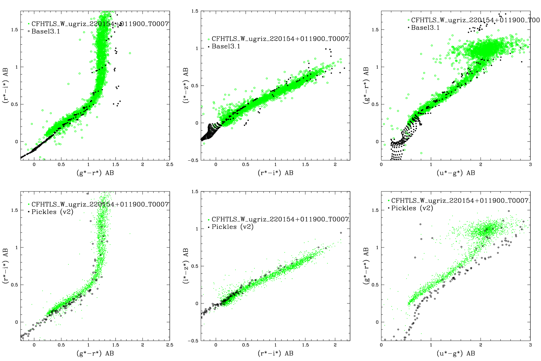
The nearly blackbody emission spectra of stars places them in a narrow line in optical and infrared color-color space. Under the assumption that stellar loci in the ugriz color space are intrinsically universal, one can identify this locus and use it to calibrate the colors (and magnitudes) of the CFHTLS sources. As in previous releases, a comparison between the CFHTLS point-source colors and stellar model tracks have been used in order to assess the stability of survey photometry from tile to tile and across the whole Wide area.

The stellar color-color loci are derived from a sample of well-defined bright stars selected from the T0007 merged catalogues. Only unsaturated objects with 17 < i < 21 and located in unmasked regions are considered (i.e. objects with FLAG==1. The MAG_AUTO as well as as the MAG_IQ20 magnitudes of the sources are plotted in the (u *-g)∕(g - r), (g - r)∕(r - i) and (r - i)∕(i - z) color-color diagrams with the color tracks of the stellar models (?).

We wish to remind the reader that the Pickles stellar library is not complete in the (T_eff ,log g) stellar parameter space, especially in the log g range. In addition, the stellar library covers only stars with solar metallicity. As shown in ?, the CFHTLS fields are a mixture of different stellar populations with different metallicities, i.e. the thin disc, the thick disc and the halo population. The effects of metallicity is largest in the (u - g) color and therefore systematic offsets compared to Pickles are to be expected. ? studied the metallicities of the CFHTLS Wide fields and they found clearly a mean metallicity below solar ([Fe/H]=-1.5). However, the metallicity variation over the Wide fields has yet to be determined.

To illustrate the effect of metallicity, Figure  38 shows the Basel 3.1 model track (?) with [Fe/H]=-1.0 (i.e. low metallically) in comparison to the Pickles models (bottom panels) with solar metallicity. While we see clearly an offset in (u - g) and (g - r) from the Pickles stars, this offset completely disappears using the Basel 3.1 [Fe/H]=-1.0 track. We therefore conclude that these offsets seen with respect to the ? stars do not represent a photometric calibration problem and can instead be explained from metallicity variations. Furthermore, realistic models of the galaxy indicate that the variations in metallicity expected in fields of sizes comparable to the CFHTLS Wide patches could correspond to displacements in color-color space of a few percent or larger,

Figure 38: Comparison of one CFHTLS field with the Pickles stellar library (lower panel) and the Basel 3.1 stellar library using [Fe/H]=-1.0 (upper panel).

4.4.7 Color offsets between CFHTLS and SDSS

In the previous CFHTLS release (T0006), the stellar locus in the Wide tiles has been used to recalibrate the photometry and improve the final field to field scatter. The differences between the loci of CFHTLS and SDSS stars in color-color tracks can be used to determine the color offsets, Δ_m-m′^SLR between the two surveys. However, as we have seen in the previous sections, the expected percent-level photometric precision of the CFHTLS Wide survey now exceeds the metallicity-induced field-to-field variations in color which we would expect in a survey the size of the CFHTLS. Consequently, this raises doubts concerning the ability of the “Stellar Locus Regression” (SLR) fitting techniques to enable further reductions in the photometric scatter of the CFHTLS wide.

To test this, we checked the potential improvement on the color offsets compared to SDSS using the SLR recalibration. First, we computed the color offsets with respect to the SDSS reference catalog δ_m-m′. We then computed the correcting color offsets from the SLR method as described in the T0006 documentation Δ^SLR_m-m′. We finally compared the rms of the color offsets across the Wide patch compared to SDSS before and after the application of the SLR corrections. Before re-calibration, the scatter in (u - g), (g - r), (r - i) and (i - z) with respect to the transformed SDSS stellar locus is 0.011, 0.005, 0.008 and 0.008 respectively; after the application of the SLR regression, this becomes 0.014, 0.011, 0.010 and 0.008.

The use of SLR clearly makes no improvement to our W3 photometric calibration, and demonstrates in our case the SLR calibration is limited to a precision larger than 1%. Without a detailed knowledge of the stellar population variations across the Wide patches, it is difficult to see how this could be improved further.

Considering the lack of improvement in the recalibration of W3 using the SLR, we chose not to use this method in T0007.