We apply a simple process to our data.

Using g-band images from the EFIGI-PGC-1.3, we first clean and rearrange them.

Then we apply the following steps:

• Compute a PCA on the pixels
• Compute the mean of the two first PC of the computed basis.
• Separate galaxies into 4 classes according to the values of their projection on the two first PC :
  • The two values are greater than the means -> subclass 11
  • Only the first value is greater than the mean -> subclass 10
  • Only the second value is greater than the mean -> subclass 01
  • None of the values is greater than the means -> subclass 00
• Repeat the same steps for each subclass

We stop when we reach a reasonible depth for the tree (4).

The results of this experiment are shown on the two following plots of the tree (three levels only). The first one depicts the Principal Components whereas the second one is the dispersion of the source on the two first PC.

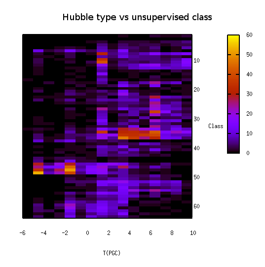
Finally, we build a tree with 4 levels and 64 leaves (classes). Then, we get the Hubble Type T for each galaxy and draw a plot to study the distribution of T amongst the classes. The following picture shows how some types are gathered together within some classes. However, the result is unusable but encouraging.

Hubble type vs. unsupervised class 64 classes (tree level 4)

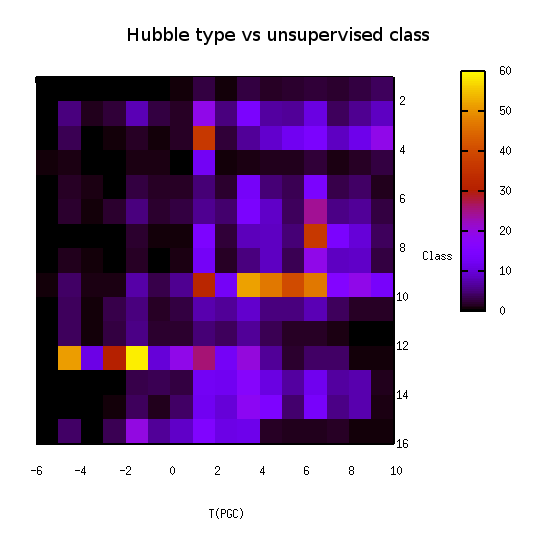
Furthermore, when we plot the same data using only 16 classes from a tree with 3 levels, the distribution is quite as precise as shown on the following picture. It suggests than an other method than a PCA should be used to go deeper than the 3rd level. It should also be more interesting to study the distribution of other attributes (bars, B/T ratio, inclination, etc) amongst the unsupervised classes.

Hubble type vs. unsupervised class 16 classes (tree level 3)